Validation

Tests check that the code does what it says; validation checks that what it says is physically and statistically right. validation/validate.py compares solvephase with theory and with an independent code. It writes a JSON report and a figure, and exits non-zero if any check fails. CI runs a reduced version on every push, and the full report is versioned in validation/artifacts.

python validation/validate.py --output validation/artifacts      # full (~2 min)
python validation/validate.py --quick --output /tmp/validation    # CI

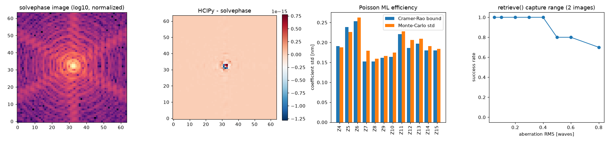
Checks and results

Check	Result	Threshold
Images vs HCIPy's Fraunhofer propagator (FFT q=2, q=3; MFT q=1.37; 3-wavelength broadband), max normalized difference	4e-16 – 4e-15	1e-10
Airy peak normalization vs \(A\theta^2/\lambda^2\) (relative)	2.2e-5	2e-3
Airy first dark ring vs \(1.22\,\lambda/D\)	0.03 λ/D (pixel 1/8 λ/D)	1/8 λ/D
Poisson ML modal estimator: Monte-Carlo variance / Cramér-Rao bound (200 noise draws, 12 modes)	1.10	0.71 – 1.40
Poisson ML estimator bias, max over modes	0.09 σ_CRB	0.85 σ_CRB
retrieve() capture with two images (±0.3 λ RMS defocus), success rate up to 0.3 waves RMS	100 % (100 % to 0.4; 80 % at 0.5–0.6; 70 % at 0.8)	100 %
Single vs double precision solution difference	8e-6 nm	0.05 nm
Phase diversity on an extended scene: relative wavefront error	3.1 %	10 %
LIFT variance / Cramér-Rao bound (150 draws)	1.01	0.68 – 1.46
Fast & Furious closed loop: residual after 20 steps / initial	0.08	0.2
CDI (HIO→ER, 4 starts) noise-free exact recovery rate	100 %	100 %
TIE (masked PCG) on a soft-edged aperture: phase error	9.6e-4 rad	0.02 rad
Reweighted amplitude flow, Gaussian model m = 8n: exact recovery rate	100 %	100 %

What the checks establish

• The forward model is right. Agreement with HCIPy, an independently written optics package, to machine precision (same orientation, sampling and normalization) covers the FFT and MFT engines and broadband summation. The Airy checks pin the absolute normalization and the sampling scale.
• The estimator is optimal. At high SNR the Poisson maximum-likelihood estimator is unbiased, and its variance equals the Cramér-Rao bound computed from the model's Fisher information (Paxman, Schulz & Fienup 1992). No unbiased estimator can do better. LIFT reaches its bound too.
• The default is robust. retrieve() recovers random aberrations from two images over the documented range without tuning. The capture curve in the figure shows where it starts to fail.
• Every family meets its documented accuracy on reference problems with known truth.

Unit tests add adjoint identities for every operator, finite-difference checks of every gradient, CPU/GPU parity, and recovery tests per algorithm (python -m pytest --run-slow --run-gpu).

Real data: Keck/NIRC2 focus diversity

Simulations can't show that a forward model matches real optics. validation/nirc2.py runs solvephase on daytime calibrations of the Keck adaptive-optics bench, taken with NIRC2's narrow camera through the full circular bench pupil. The script uses no data that would need an outside calibration. Each run is a stack of nine H-band (1.6455 µm) images at focus-stage offsets from −7 to +2.5. In six runs, a known pattern was added to the 349-actuator Xinetics DM command: coma, or coma plus trefoil at three strengths.

The data belong to the observatory and are not distributed with solvephase. The committed report and figures come from

python validation/nirc2.py --data /path/to/image_sharpening_datasets --output validation/artifacts

which takes about 3 minutes (--quick takes about 1 minute).

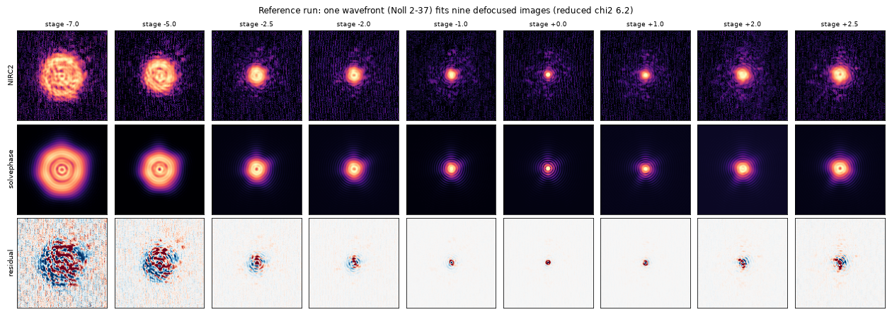
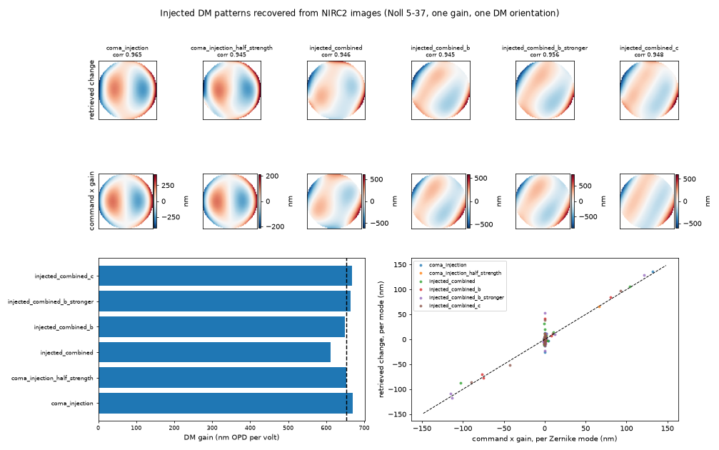
Check	Result	Threshold
One wavefront (Noll 2–37) fits all nine images of a run: reduced χ²	4.1 – 7.7	≤ 10
Injection minus reference recovers the commanded DM pattern (Noll 5–37): correlation, each of 6 runs	0.945 – 0.965	≥ 0.90
One DM gain explains every run: run-to-run scatter	3.0 % (652 nm OPD per volt)	≤ 10 %
Half-strength coma / full coma (needs no gain)	0.499 (commanded 0.500)	±10 %
Stronger / base combined injection (needs no gain)	1.517 (commanded 1.500)	±10 %
Wavefront change from the IDL sharpening correction, predicted from its DM command with no free parameter: correlation	0.90	≥ 0.85
Same prediction: measured / predicted amplitude	0.994	±20 %
DM gain across fits with 21, 28 and 36 modes	0.4 %	≤ 5 %
DM gain vs the Keck AO software's 600 nm/V	652 nm/V (+8.7 %)	±15 %
Fitted pupil radius vs the Xinetics control aperture (5.52 in at 7 mm pitch = 10.0 pitches)	9.75 pitches (−2.6 %)	±5 %

How it works:

• Calibration. Two scalars are fitted once on the reference run by profile likelihood: the RMS defocus per focus-stage unit (190 nm) and the sampling (3.15 px per λ/D). The nominal sampling for a 10.95 m aperture at 9.971 mas/pixel is 3.11 px per λ/D. Every other run reuses both values.
• Retrieval. Each run is fitted with FocalPlaneProblem: a circular pupil, 36 Zernike modes, a Gaussian likelihood with photon and read-noise weights, and per-frame flux, background and tip/tilt. Each frame is cropped around its own centroid, so tip, tilt and focus are left out of run-to-run comparisons.
• DM geometry. One orientation of the 21×21 actuator grid fits every run: a reflection, a −2° rotation, and a pupil radius of 9.75 actuator pitches. It is fitted once by correlation over all six injections. The flip that fits the coma runs alone fails on the trefoil runs, so the combination pins it down.

What it shows: with only two calibration scalars, solvephase's physical model turns real, noisy, detector-limited images into wavefronts. Those wavefronts are linear in the commanded DM shape (the strength ratios), and they are consistent between runs (one gain, one geometry). They also predict an independent correction they were never fitted to. Both the DM gain and the pupil size agree with the Keck AO software's Xinetics parameters, which the fit never sees. The 600 nm/V conversion therefore converts wavefront (OPD), not mirror surface.

Limits on these data:

• The residual images show structure the 36-mode model doesn't capture: fine speckle in the far-defocused frames, a slightly sharper in-focus core, and detector column stripes.
• Fits with 55 modes are not identifiable. Solutions about 300 nm RMS apart differ by only a few per cent in χ², so the injection checks degrade there. This points to unmodelled pupil illumination and detector structure leaking into high-order modes, not to a solver failure: regularization and an orthonormalized basis leave it unchanged, while 21 to 36 modes agree.