Validation

pyturb's turbulence is checked against analytic theory, not just asserted to be correct. validation/validate.py regenerates the figure below and prints a PASS/FAIL for each check against its tolerance; it runs in a few seconds and is suitable for CI.

python validation/validate.py

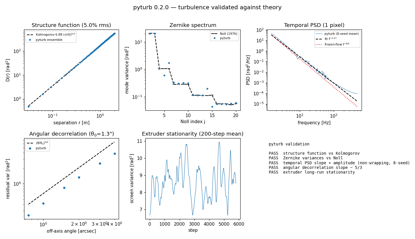
What each panel shows

Structure function vs Kolmogorov. The azimuthally-averaged phase structure function of an ensemble of FFT screens (subharmonic-corrected) matches D(r) = 6.88 (r/r0)^{5/3} to a few percent across the inertial range at separations of a few pixels and up — the core check that the spatial statistics are right. The 1-2 pixel (near-Nyquist) scales show a larger deficit (order 5-10%) from finite grid sampling, so read the "few percent" figure with a

~2-4 pixel resolution qualifier at the shortest scale of interest.

Zernike spectrum vs Noll (1976). Screens are decomposed with pyturb.analysis.zernike_decompose and the per-mode variances compared to the Kolmogorov values Δ_{j-1} − Δ_j of Noll. The aggregate over modes agrees to ~10%. (Finite screens under-sample tip/tilt, and a square grid splits the two astigmatism modes — both are real sampling effects, visible as the small per-mode scatter.)

Temporal PSD. The time series of a single pupil pixel under frozen flow follows the f^{-8/3} power law in the inertial regime; the bumps are the wind-crossing harmonics of the finite aperture. Fit with analysis.temporal_psd + analysis.fit_power_law.

Angular decorrelation. The residual variance between the on-axis and an off-axis line of sight grows as (θ/θ0)^{5/3} near the isoplanatic angle (analysis.differential_variance), confirming the geometry of the off-axis directions= path. Well beyond θ0 the curve saturates as the two footprints fully decorrelate.

Extruder stationarity. The variance of an InfinitePhaseScreen shows no secular drift over thousands of steps (guarding against conditional-covariance error accumulation). The fast wiggle is the physical beating of the few large-scale modes a small screen contains, not drift.

Finite-screen resolution. The structure-function/theory ratio at 1, 2, 4, and 8 pixels makes the documented near-Nyquist finite-grid deficit explicit; the resolved 4–8 pixel scales remain close to theory.

Zenith projection. The scalar airmass approximation is checked directly: r0 scales as cos(z)^(3/5), layer range as sec(z), and therefore theta0 as cos(z)^(8/5). This validates the implemented scalar model, not an anisotropic slant-path coordinate transform.

Reproducing

The script uses only pyturb, NumPy and Matplotlib, and by default writes docs/images/validation.png. For CI or an experiment, keep generated evidence out of the worktree with --output and record the per-check results with --metrics:

python validation/validate.py --output /tmp/validation.png \
    --metrics /tmp/validation.json

The JSON records the command, UTC generation time, installed pyturb version, and GitHub Actions revision (or the local Git commit when available), alongside the individual check results. A source_dirty flag makes it clear when a local artifact was produced from uncommitted source changes.

Every check is an ensemble comparison to a closed form, so re-running with a different seed gives the same conclusions within the stated tolerances. The same primitives (pyturb.analysis) are available to build your own diagnostics — see interop.